To cluster a protein conformations using distance-matrix PCA
In this tutorial, conformational clustering of a flexible protein TFAM will be performed using the distance-matrix PCA (dmPCA). TFAM is a mitochondiral protein that interact and binds with the mitochondiral DNA. When TFAM is bound to the DNA, its conformation is rigid, however, in unbound form TFAM is extremely flexible.
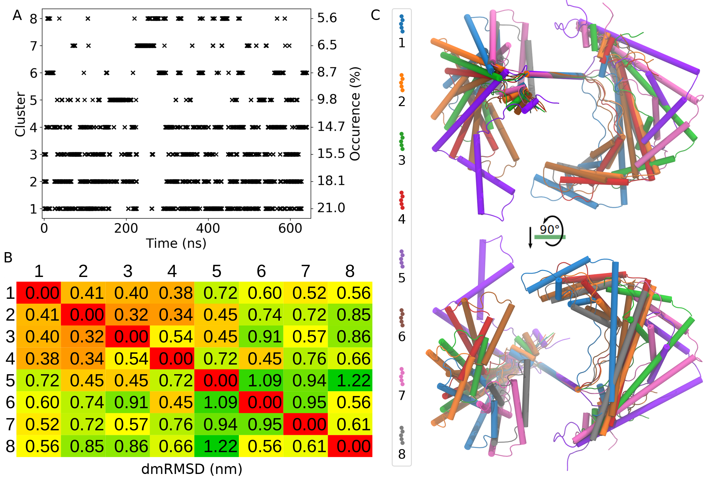
Final result
Instructions
Tutorial files: The tutorial files can be downloaded from here.
Extract the files:
tar -zxvf distmat-TFAM-pca.tar.gzGo to directory:
cd distmat-TFAM-pcaCopy the Jupyter Notebook: This notebook is available in the GitHub repo. Download and copy it from the github.
Required Tools
GROMACS
gmx_clusterByFeatures
Steps
Since the conformations are flexible, the fitting or superimposition is not accurate with the reference structure, therefore cartesian-coordinate PCA is not enough to accurately cluster the conformation. Instead we will employ distance-matrix based PCA to cluster the conformations of the TFAM. Following steps will be performed to do clustering:
Calculation of distance-matrix over the trajectory
PCA from the distance-matrix
Calculation of Projections of first ten PCs on the trajectory
Clustering using first ten PCs as the features
Analysis
1. Calculation of distance-matrix over the trajectory
We will use distmat sub-command to calculate the distance-matrix over the trajectory. Following command will generate two files:
pca.xtc: This file is acontainerfor distance-matrices over the entire trajectory inxtcfile format. This is not a real trajectory file.pca_dummy.pdb: This is a dummy pdb file containing same number of entries as obtained in above xtc file.
Notes
-gx 5is used to reduce the size of distance-matrix. It means that there is a gap of 4 residues along X-axis in distance-matrix. For example, if a protein contains 100 residues, distance-matrix size is 100x100. If -gx 5 is used, new size is 20x100.-gxand-gyoptions ONLY affect output produced with-pcaoption ofdistmat.The distance-matrix calculation is parallelized using pthread, and therefore will use all the available threads of the CPU. It can be controlled using
-ntoption.
[1]:
%%bash

echo 3 3 | gmx_clusterByFeatures distmat -f inputs/woDNA.xtc -s inputs/woDNA.tpr -n inputs/index.ndx -pca -gx 5 -std stdev-matrix.dat
 :-) GROMACS - gmx_clusterByFeatures distmat, 2025.0-dev-20250210-6949615-local (-:

Executable:   gmx_clusterByFeatures distmat
Data prefix:  /project/external/gmx_installed
Working dir:  /home/raj/workspace/gmx_clusterByFeatrues/tutorials/distmat-TFAM-pca
Command line:
  'gmx_clusterByFeatures distmat' -f inputs/woDNA.xtc -s inputs/woDNA.tpr -n inputs/index.ndx -pca -gx 5 -std stdev-matrix.dat


         :-)  gmx_clusterByFeatures distmat (-:

             Author: Rajendra Kumar

       Copyright (C) 2018-2019  Rajendra Kumar


gmx_clusterByFeatures is a free software: you can redistribute it and/or modify
it under the terms of the GNU General Public License as published by
the Free Software Foundation, either version 3 of the License, or
(at your option) any later version.

gmx_clusterByFeatures is distributed in the hope that it will be useful,
but WITHOUT ANY WARRANTY; without even the implied warranty of
MERCHANTABILITY or FITNESS FOR A PARTICULAR PURPOSE.  See the
GNU General Public License for more details.

You should have received a copy of the GNU General Public License
along with gmx_clusterByFeatures.  If not, see <http://www.gnu.org/licenses/>.

THIS SOFTWARE IS PROVIDED BY THE COPYRIGHT HOLDERS AND CONTRIBUTORS
"AS IS" AND ANY EXPRESS OR IMPLIED WARRANTIES, INCLUDING, BUT NOT
LIMITED TO, THE IMPLIED WARRANTIES OF MERCHANTABILITY AND FITNESS FOR
A PARTICULAR PURPOSE ARE DISCLAIMED. IN NO EVENT SHALL THE COPYRIGHT
OWNER OR CONTRIBUTORS BE LIABLE FOR ANY DIRECT, INDIRECT, INCIDENTAL,
SPECIAL, EXEMPLARY, OR CONSEQUENTIAL DAMAGES (INCLUDING, BUT NOT LIMITED
TO, PROCUREMENT OF SUBSTITUTE GOODS OR SERVICES; LOSS OF USE, DATA, OR
PROFITS; OR BUSINESS INTERRUPTION) HOWEVER CAUSED AND ON ANY THEORY OF
LIABILITY, WHETHER IN CONTRACT, STRICT LIABILITY, OR TORT (INCLUDING
NEGLIGENCE OR OTHERWISE) ARISING IN ANY WAY OUT OF THE USE OF THIS
SOFTWARE, EVEN IF ADVISED OF THE POSSIBILITY OF SUCH DAMAGE.

Reading file inputs/woDNA.tpr, VERSION 4.5.5-dev-20110921-e25c350 (single precision)
Reading file inputs/woDNA.tpr, VERSION 4.5.5-dev-20110921-e25c350 (single precision)
Select first group:
Group     0 (         System) has  3580 elements
Group     1 (        Protein) has  3580 elements
Group     2 (      Protein-H) has  1884 elements
Group     3 (        C-alpha) has   195 elements
Group     4 (       Backbone) has   585 elements
Group     5 (      MainChain) has   781 elements
Group     6 (   MainChain+Cb) has   973 elements
Group     7 (    MainChain+H) has   969 elements
Group     8 (      SideChain) has  2611 elements
Group     9 (    SideChain-H) has  1103 elements
Group    10 (    Prot-Masses) has  3338 elements
Group    11 (r_16-25_r_35-45_r_52-75_r_82-110_r_120-130_r_136-145_r_152-180) has  2331 elements
Group    12 (r_16-25_r_35-45_r_52-75_r_82-110_r_120-130_r_136-145_r_152-180_&_C-alpha) has   124 elements
Group    13 (r_1-98_&_C-alpha) has    98 elements
Group    14 (r_99-195_&_C-alpha) has    97 elements
Select a group: Select second group:
Group     0 (         System) has  3580 elements
Group     1 (        Protein) has  3580 elements
Group     2 (      Protein-H) has  1884 elements
Group     3 (        C-alpha) has   195 elements
Group     4 (       Backbone) has   585 elements
Group     5 (      MainChain) has   781 elements
Group     6 (   MainChain+Cb) has   973 elements
Group     7 (    MainChain+H) has   969 elements
Group     8 (      SideChain) has  2611 elements
Group     9 (    SideChain-H) has  1103 elements
Group    10 (    Prot-Masses) has  3338 elements
Group    11 (r_16-25_r_35-45_r_52-75_r_82-110_r_120-130_r_136-145_r_152-180) has  2331 elements
Group    12 (r_16-25_r_35-45_r_52-75_r_82-110_r_120-130_r_136-145_r_152-180_&_C-alpha) has   124 elements
Group    13 (r_1-98_&_C-alpha) has    98 elements
Group    14 (r_99-195_&_C-alpha) has    97 elements
Select a group: There are 195 residues with 195 atoms in first group
There are 195 residues with 195 atoms in second group
Reading frame   32000 time 640000.000

GROMACS reminds you: "The Feeling of Power was Intoxicating, Magic" (Frida Hyvonen)
Selected 3: 'C-alpha'
Selected 3: 'C-alpha'
 Number of distance-matrix elements for PCA trajectory: 3706
 Number of distance-matrix coordinates in PCA trajectory: 1236
2. PCA from the distance-matrix
Now, we will use pca.xtc and pca_dummy.pdb generated in the above command as input files to GROMACS tool gmx covar to perform PCA. This step will calculate covariance matrix, eigenvectors and eigenvalues. By default, the eigenvectors are written in eigenvec.trr while eigenvalues are written in eigenval.xvg files.
-nofit, -nomwa and -nopbc options are used because xtc file does not contain cartesian-coordinates and these option has no meanings in the case of the distance-matrix trajectory.
[2]:
%%bash

echo 0 | gmx covar -f pca.xtc -s pca_dummy.pdb -nofit -nomwa -nopbc
                      :-) GROMACS - gmx covar, 2025.2 (-:

Executable:   /opt/gromacs-2025/bin/gmx
Data prefix:  /opt/gromacs-2025
Working dir:  /home/raj/workspace/gmx_clusterByFeatrues/tutorials/distmat-TFAM-pca
Command line:
  gmx covar -f pca.xtc -s pca_dummy.pdb -nofit -nomwa -nopbc

Group     0 (         System) has  1236 elements
Group     1 (        Protein) has  1236 elements
Group     2 (      Protein-H) has  1236 elements
Group     3 (        C-alpha) has  1236 elements
Group     4 (       Backbone) has  1236 elements
Group     5 (      MainChain) has  1236 elements
Group     6 (   MainChain+Cb) has  1236 elements
Group     7 (    MainChain+H) has  1236 elements
Group     8 (      SideChain) has     0 elements
Group     9 (    SideChain-H) has     0 elements
Select a group: Calculating the average structure ...
Reading frame   32000 time 640000.000
Constructing covariance matrix (3708x3708) ...
Reading frame   32000 time 640000.000
Read 32016 frames

Trace of the covariance matrix: 803.441 (nm^2)

Diagonalizing ...

Sum of the eigenvalues: 803.442 (nm^2)

Writing eigenvalues to eigenval.xvg

Writing average structure & eigenvectors 1--3708 to eigenvec.trr
Wrote the log to covar.log

GROMACS reminds you: "Courage is like - it's a habitus, a habit, a virtue: you get it by courageous acts. It's like you learn to swim by swimming. You learn courage by couraging." (Marie Daly)
WARNING: Masses and atomic (Van der Waals) radii will be guessed
         based on residue and atom names, since they could not be
         definitively assigned from the information in your input
         files. These guessed numbers might deviate from the mass
         and radius of the atom type. Please check the output
         files if necessary. Note, that this functionality may
         be removed in a future GROMACS version. Please, consider
         using another file format for your input.


Choose a group for the covariance analysis
Selected 0: 'System'
3. Projections of first ten PCs on the trajectory
We will use eigenvectors written in eigenvec.trr, pca.xtc and pca_dummy.pdb as input files to GROMACS tool gmx anaeig to calculate projection of first 10 eigenvectors on distance-matrix trajectory. These projections will be written into proj.xvg file.
[3]:
%%bash

echo 0 0 | gmx anaeig -f pca.xtc -s pca_dummy.pdb -first 1 -last 10 -proj
                      :-) GROMACS - gmx anaeig, 2025.2 (-:

Executable:   /opt/gromacs-2025/bin/gmx
Data prefix:  /opt/gromacs-2025
Working dir:  /home/raj/workspace/gmx_clusterByFeatrues/tutorials/distmat-TFAM-pca
Command line:
  gmx anaeig -f pca.xtc -s pca_dummy.pdb -first 1 -last 10 -proj

trr version: GMX_trn_file (single precision)
Eigenvectors in eigenvec.trr were determined without fitting
Read non mass weighted average/minimum structure with 1236 atoms from eigenvec.trr
Read 3708 eigenvectors (for 1236 atoms)


WARNING: If there are molecules in the input trajectory file
         that are broken across periodic boundaries, they
         cannot be made whole (or treated as whole) without
         you providing a run input file.

Group     0 (         System) has  1236 elements
Group     1 (        Protein) has  1236 elements
Group     2 (      Protein-H) has  1236 elements
Group     3 (        C-alpha) has  1236 elements
Group     4 (       Backbone) has  1236 elements
Group     5 (      MainChain) has  1236 elements
Group     6 (   MainChain+Cb) has  1236 elements
Group     7 (    MainChain+H) has  1236 elements
Group     8 (      SideChain) has     0 elements
Group     9 (    SideChain-H) has     0 elements
Select a group: 10 eigenvectors selected for output: 1 2 3 4 5 6 7 8 9 10
Reading frame   32000 time 640000.000


GROMACS reminds you: "Courage is like - it's a habitus, a habit, a virtue: you get it by courageous acts. It's like you learn to swim by swimming. You learn courage by couraging." (Marie Daly)
Select an index group of 1236 elements that corresponds to the eigenvectors
Selected 0: 'System'
4. Clustering using first ten PCs
Now, we will perform clustering using K-Means algorithm. One of the drawback of K-Means clustering is that the number of clusters should be known beforehand. To automate the decision about number of clusters, gmx_clusterByFeatures implements several cluster metrics. We will use option -cmetric ssr-sst to use the [Elbow
method](https://en.wikipedia.org/wiki/Elbow_method_(clustering).
Following command will perform the clustering of conformations using firt 10 PCs projection. Explanation of options are as follows:
-method kmeans: Use K-Means clustering algorithm-ncluster 10: K-Means clustering will be performed for 1 upto 10 clusters times each time. Finally, based on-ssrchangeoption, final number of clusters will be automatically selected.-cmetric ssr-sst: Use Elbow method to decide final number of clusters.-nfeature 10: Take 10 feature fromfeat proj.xvginput file. Here it is projection of first ten eigenvectors.-sort features: Sort the output clustered trajectory based on the distance in feature space from its central structure.-fit2central: Fit/Superimpose the conformation on central structure in output clustered trajectory.-ssrchange 2: Threshold (percentage) of change in SSR/SST ratio in Elbow method to decide the number of clusters.-cpdb clustered-trajs/central.pdb: Dump central conformation of each cluster as a separate pdb file.-fout clustered-trajs/cluster.xtc: Dump conformations of each cluster as the separate trajectory file.-plot pca_cluster.png: Plot the feature-space (here, it is first 10 PCs from PCA) coloured by the clusters.-rmsd clustered-trajs/rmsd.xvg: Calculate the RMSD with reference to central conformation of each clusters and written in separate files.
index group order
First index group - Output group of atoms in the central structures and clustered trajectories
Second index group - Group of atoms to calculate distance-matrix RMSD between central conformations of clusters as RMSD matrix, which is dumped in the log file with
-goption. Here, it is C-alpha atoms of protein.Third index group - Used for Superimposition by least-square fitting. ONLY used in separate clustered trajectories to superimpose conformations on the central structure.
Note: This command could take a long time to execute!
This command could take a long time to execute because it is writing output trajectory file for each cluster sorted by distance in feature-space. Therefore, it needs to read input trajectory back-and-forth many time to extract the conformations in sorted manner. XTC format is fast for back-and-forth reading, and it still could take long time to dump the output trajectories.
Content of output ``-g cluster.log`` file
It contains the command summary, and for each input cluster-numbers, number of frames in each clusters. At the end, it contains the Cluster Metrics Summary, which is important for deciding final number of clusters.
[ ]:
%%bash

# create a new folder to contain clustered trajectory and pdb files
mkdir clustered-trajs

echo 0 3 3 | gmx_clusterByFeatures cluster -s inputs/woDNA.tpr -f inputs/woDNA.xtc -n inputs/index.ndx -feat proj.xvg -method kmeans \
                                           -nfeature 10 -cmetric ssr-sst -ncluster 20 -fit2central -sort rmsdist \
                                           -ssrchange 2 -cpdb clustered-trajs/central.pdb -fout clustered-trajs/cluster.xtc \
                                           -plot pca_cluster.png
 :-) GROMACS - gmx_clusterByFeatures cluster, 2025.0-dev-20250210-6949615-local (-:

Executable:   gmx_clusterByFeatures cluster
Data prefix:  /project/external/gmx_installed
Working dir:  /home/raj/workspace/gmx_clusterByFeatrues/tutorials/distmat-TFAM-pca
Command line:
  'gmx_clusterByFeatures cluster' -s inputs/woDNA.tpr -f inputs/woDNA.xtc -n inputs/index.ndx -feat proj.xvg -method kmeans -nfeature 10 -cmetric ssr-sst -ncluster 20 -fit2central -sort rmsdist -ssrchange 2 -cpdb clustered-trajs/central.pdb -fout clustered-trajs/cluster.xtc -plot pca_cluster.png


         :-)  gmx_clusterByFeatures cluster (-:

             Author: Rajendra Kumar

       Copyright (C) 2018-2019  Rajendra Kumar


gmx_clusterByFeatures is a free software: you can redistribute it and/or modify
it under the terms of the GNU General Public License as published by
the Free Software Foundation, either version 3 of the License, or
(at your option) any later version.

gmx_clusterByFeatures is distributed in the hope that it will be useful,
but WITHOUT ANY WARRANTY; without even the implied warranty of
MERCHANTABILITY or FITNESS FOR A PARTICULAR PURPOSE.  See the
GNU General Public License for more details.

You should have received a copy of the GNU General Public License
along with gmx_clusterByFeatures.  If not, see <http://www.gnu.org/licenses/>.

THIS SOFTWARE IS PROVIDED BY THE COPYRIGHT HOLDERS AND CONTRIBUTORS
"AS IS" AND ANY EXPRESS OR IMPLIED WARRANTIES, INCLUDING, BUT NOT
LIMITED TO, THE IMPLIED WARRANTIES OF MERCHANTABILITY AND FITNESS FOR
A PARTICULAR PURPOSE ARE DISCLAIMED. IN NO EVENT SHALL THE COPYRIGHT
OWNER OR CONTRIBUTORS BE LIABLE FOR ANY DIRECT, INDIRECT, INCIDENTAL,
SPECIAL, EXEMPLARY, OR CONSEQUENTIAL DAMAGES (INCLUDING, BUT NOT LIMITED
TO, PROCUREMENT OF SUBSTITUTE GOODS OR SERVICES; LOSS OF USE, DATA, OR
PROFITS; OR BUSINESS INTERRUPTION) HOWEVER CAUSED AND ON ANY THEORY OF
LIABILITY, WHETHER IN CONTRACT, STRICT LIABILITY, OR TORT (INCLUDING
NEGLIGENCE OR OTHERWISE) ARISING IN ANY WAY OUT OF THE USE OF THIS
SOFTWARE, EVEN IF ADVISED OF THE POSSIBILITY OF SUCH DAMAGE.

Reading file inputs/woDNA.tpr, VERSION 4.5.5-dev-20110921-e25c350 (single precision)
Reading file inputs/woDNA.tpr, VERSION 4.5.5-dev-20110921-e25c350 (single precision)
Group     0 (         System) has  3580 elements
Group     1 (        Protein) has  3580 elements
Group     2 (      Protein-H) has  1884 elements
Group     3 (        C-alpha) has   195 elements
Group     4 (       Backbone) has   585 elements
Group     5 (      MainChain) has   781 elements
Group     6 (   MainChain+Cb) has   973 elements
Group     7 (    MainChain+H) has   969 elements
Group     8 (      SideChain) has  2611 elements
Group     9 (    SideChain-H) has  1103 elements
Group    10 (    Prot-Masses) has  3338 elements
Group    11 (r_16-25_r_35-45_r_52-75_r_82-110_r_120-130_r_136-145_r_152-180) has  2331 elements
Group    12 (r_16-25_r_35-45_r_52-75_r_82-110_r_120-130_r_136-145_r_152-180_&_C-alpha) has   124 elements
Group    13 (r_1-98_&_C-alpha) has    98 elements
Group    14 (r_99-195_&_C-alpha) has    97 elements
Select a group: Group     0 (         System) has  3580 elements
Group     1 (        Protein) has  3580 elements
Group     2 (      Protein-H) has  1884 elements
Group     3 (        C-alpha) has   195 elements
Group     4 (       Backbone) has   585 elements
Group     5 (      MainChain) has   781 elements
Group     6 (   MainChain+Cb) has   973 elements
Group     7 (    MainChain+H) has   969 elements
Group     8 (      SideChain) has  2611 elements
Group     9 (    SideChain-H) has  1103 elements
Group    10 (    Prot-Masses) has  3338 elements
Group    11 (r_16-25_r_35-45_r_52-75_r_82-110_r_120-130_r_136-145_r_152-180) has  2331 elements
Group    12 (r_16-25_r_35-45_r_52-75_r_82-110_r_120-130_r_136-145_r_152-180_&_C-alpha) has   124 elements
Group    13 (r_1-98_&_C-alpha) has    98 elements
Group    14 (r_99-195_&_C-alpha) has    97 elements
Reading frame       4 time   80.000
=======================
  Cluster Log output
=======================

Command:
=======================
'gmx_clusterByFeatures cluster' -s inputs/woDNA.tpr -f inputs/woDNA.xtc -n inputs/index.ndx -feat proj.xvg -method kmeans -nfeature 10 -cmetric ssr-sst -ncluster 20 -fit2central -sort rmsdist -ssrchange 2 -cpdb clustered-trajs/central.pdb -fout clustered-trajs/cluster.xtc -plot pca_cluster.png
=======================

Choose a group for the output:
Selected 0: 'System'

Choose a group for clustering/RMSD calculation:
Selected 3: 'C-alpha'

Choose a group for fitting or superposition:
Selected 3: 'C-alpha'


 Input Trajectory dt = 20 ps


###########################################
########## NUMBER OF CLUSTERS : 1 ########
###########################################

===========================
Cluster-ID      TotalFrames
1               32016
===========================


###########################################
########## NUMBER OF CLUSTERS : 2 ########
###########################################

===========================
Cluster-ID      TotalFrames
1               16361
2               15655
===========================


###########################################
########## NUMBER OF CLUSTERS : 3 ########
###########################################

===========================
Cluster-ID      TotalFrames
1               11769
2               11232
3               9015
===========================


###########################################
########## NUMBER OF CLUSTERS : 4 ########
###########################################

===========================
Cluster-ID      TotalFrames
1               14782
2               6838
3               6711
4               3685
===========================


###########################################
########## NUMBER OF CLUSTERS : 5 ########
###########################################

===========================
Cluster-ID      TotalFrames
1               11103
2               8298
3               4572
4               4469
5               3574
===========================


###########################################
########## NUMBER OF CLUSTERS : 6 ########
###########################################

===========================
Cluster-ID      TotalFrames
1               10817
2               8501
3               4195
4               3453
5               3117
6               1933
===========================


###########################################
########## NUMBER OF CLUSTERS : 7 ########
###########################################

===========================
Cluster-ID      TotalFrames
1               7022
2               6867
3               6716
4               4211
5               3361
6               2132
7               1707
===========================


###########################################
########## NUMBER OF CLUSTERS : 8 ########
###########################################

===========================
Cluster-ID      TotalFrames
1               6783
2               5835
3               4901
4               4757
5               3120
6               2781
7               2043
8               1796
===========================


###########################################
########## NUMBER OF CLUSTERS : 9 ########
###########################################

===========================
Cluster-ID      TotalFrames
1               6175
2               5059
3               4361
4               4350
5               3074
6               2767
7               2476
8               2040
9               1714
===========================


###########################################
########## NUMBER OF CLUSTERS : 10 ########
###########################################

===========================
Cluster-ID      TotalFrames
1               4994
2               4179
3               3965
4               3882
5               3618
6               2685
7               2623
8               2473
9               1988
10              1609
===========================


###########################################
########## NUMBER OF CLUSTERS : 11 ########
###########################################

===========================
Cluster-ID      TotalFrames
1               4465
2               3960
3               3851
4               3330
5               3283
6               2662
7               2622
8               2506
9               1946
10              1878
11              1513
===========================


###########################################
########## NUMBER OF CLUSTERS : 12 ########
###########################################

===========================
Cluster-ID      TotalFrames
1               4370
2               4069
3               4000
4               3629
5               3293
6               2108
7               2038
8               1934
9               1872
10              1814
11              1478
12              1411
===========================


###########################################
########## NUMBER OF CLUSTERS : 13 ########
###########################################

===========================
Cluster-ID      TotalFrames
1               3456
2               3334
3               3306
4               3256
5               3109
6               2748
7               2350
8               2327
9               1940
10              1803
11              1657
12              1432
13              1298
===========================


###########################################
########## NUMBER OF CLUSTERS : 14 ########
###########################################

===========================
Cluster-ID      TotalFrames
1               3629
2               3217
3               2921
4               2887
5               2846
6               2839
7               2429
8               1837
9               1762
10              1744
11              1743
12              1547
13              1378
14              1237
===========================


###########################################
########## NUMBER OF CLUSTERS : 15 ########
###########################################

===========================
Cluster-ID      TotalFrames
1               3666
2               3233
3               3217
4               3012
5               2987
6               2790
7               1906
8               1718
9               1603
10              1479
11              1342
12              1286
13              1281
14              1255
15              1241
===========================


###########################################
########## NUMBER OF CLUSTERS : 16 ########
###########################################

===========================
Cluster-ID      TotalFrames
1               3524
2               3309
3               2865
4               2841
5               2744
6               2651
7               2305
8               1745
9               1568
10              1436
11              1337
12              1263
13              1236
14              1197
15              1160
16              835
===========================


###########################################
########## NUMBER OF CLUSTERS : 17 ########
###########################################

===========================
Cluster-ID      TotalFrames
1               3192
2               2864
3               2849
4               2579
5               2405
6               2366
7               2259
8               1904
9               1602
10              1528
11              1468
12              1373
13              1349
14              1169
15              1168
16              1012
17              929
===========================


###########################################
########## NUMBER OF CLUSTERS : 18 ########
###########################################

===========================
Cluster-ID      TotalFrames
1               3326
2               2848
3               2777
4               2575
5               2479
6               2444
7               2109
8               1532
9               1483
10              1455
11              1356
12              1334
13              1202
14              1172
15              1160
16              1018
17              928
18              818
===========================


###########################################
########## NUMBER OF CLUSTERS : 19 ########
###########################################

===========================
Cluster-ID      TotalFrames
1               3158
2               2785
3               2657
4               2474
5               2447
6               2361
7               2211
8               1531
9               1444
10              1393
11              1362
12              1349
13              1255
14              1234
15              1159
16              1011
17              921
18              803
19              461
===========================


###########################################
########## NUMBER OF CLUSTERS : 20 ########
###########################################

===========================
Cluster-ID      TotalFrames
1               2566
2               2549
3               2314
4               2285
5               2260
6               2216
7               2025
8               1777
9               1489
10              1469
11              1443
12              1324
13              1158
14              1157
15              1119
16              1115
17              1102
18              988
19              909
20              751
===========================


===========================================================================================================
                                          Cluster Metrics Summary
-----------------------------------------------------------------------------------------------------------
Clusters       SSR/SST    D(SSR/SST)         (Psuedo)F-stat.    Silhouette-score   Davies-bouldin-score
2              31.27      31.268                  14563.710     0.262              1.381
3              44.44      13.173                  12803.176     0.228              1.406
4              52.77       8.332                  11923.432     0.234              1.306
5              57.66       4.885                  10897.036     0.203              1.391
6              61.47       3.816                  10214.958     0.211              1.345
7              64.70       3.222                   9775.873     0.206              1.339
8              66.75       2.057                   9180.444     0.191              1.398
9              68.29       1.540                   8616.962     0.188              1.428
10             69.71       1.420                   8185.188     0.182              1.403
11             70.90       1.193                   7799.618     0.183              1.396
12             72.00       1.095                   7481.315     0.181              1.486
13             72.84       0.841                   7152.562     0.179              1.432
14             73.87       1.033                   6960.579     0.179              1.424
15             74.69       0.816                   6745.368     0.178              1.446
16             75.54       0.849                   6588.000     0.181              1.416
17             76.10       0.559                   6367.346     0.182              1.404
18             76.89       0.793                   6262.695     0.180              1.407
19             77.40       0.508                   6087.359     0.181              1.387
20             77.92       0.521                   5942.556     0.182              1.411
===========================================================================================================


#####################################
Final number of cluster selected: 8
#####################################

Calculating central structure for cluster-8 ...
Reading frame       7 time 274760.000   <string>:127: MatplotlibDeprecationWarning: The non_interactive_bk attribute was deprecated in Matplotlib 3.9 and will be removed in 3.11. Use ``matplotlib.backends.backend_registry.list_builtin(matplotlib.backends.BackendFilter.NON_INTERACTIVE)`` instead.
Reading frame    2000 time 220340.000
5. Analysis
Now, we will perform following analysis on obtained clusters:
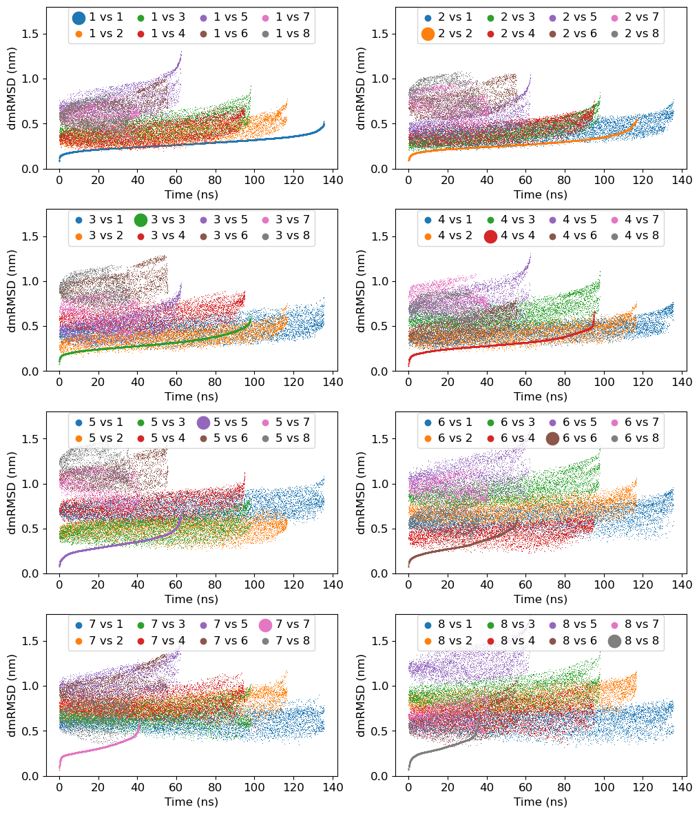
Comparison of Distance-Matrix-RMSDs within and between the clusters: It will highlight the quality of clustering by measuring the difference in the clusters using distance-matrix RMSD
Plotting PC vs PC cluster-wise. In fact, this is already plotted in the above obtained
pca_cluster.pngfile. However, we will focus on first three PCs to demonstrate the distribution of conformation in PC space.Plotting distance-matrix-RMSF: Because, we are calculating distance-matrix over the trajectory, it gives us another way to compute RMSF by using distance-matrix. To gain insight of the flexible and rigid regions of the protein, this analysis is useful. It is similar to RMSF but avoids structure fitting and therefore, suitable for highly flexible proteins.
Cluster-ID with time: We will plot cluster-id as a function of time to analyze, how conformation is changing between clusters as a function of time.
At first, we will load Python modules and define some functions as follows:
[13]:
import re
import sys
import numpy as np
import matplotlib as mpl
import matplotlib.pyplot as plt
[14]:
def read_mat_file(filename):
    ''' Read the matrix file generated from distmat sub-command
    '''
    fin = open(filename, 'r')

    data = []
    for line in fin:
        line = line.rstrip().lstrip()
        if not line:
            continue

        temp = re.split('\s+', line)
        data.append(list(map(float, temp)))

    data = np.asarray(data)

    return data.T

def read_xvg(filename):
    ''' Read any XVG file and return the data as 2D array where data is row-wise with respect to time.
    '''
    fin = open(filename, 'r')

    data = []
    for line in fin:
        line = line.rstrip().lstrip()
        if not line:
            continue

        if re.search('^#|^@', line) is not None:
                     continue

        temp = re.split('\s+', line)
        data.append(list(map(float, temp)))

    data = np.asarray(data)

    return data.T
1a. Calculation of Distance-Matrix-RMSDs within and between the clusters
At first, we need to calculate distance-matrix RMSD within and between the clusters using gmx rmsdist command as follows.
Note: Remove %%capture --no-stdout and %%capture --no-stderr to populate all the output generated from gmx rmsdist commands.
[15]:
%%capture --no-stdout
%%capture --no-stderr
%%script bash

mkdir rmsdist

# Nested For loop to calculate rmsdist of clustered-trajectory with reference to central structure with all possible combinations.
for i in `seq 1 8`
do
    for j in `seq 1 8`
    do
        echo 3 | gmx rmsdist -f clustered-trajs/cluster_c${j}.xtc -s clustered-trajs/central_c${i}.pdb -o rmsdist/c${i}_c${j} -nopbc
    done
done
1b. Comparison of Distance-Matrix-RMSDs within and between the clusters
We will use Python to plot all the obtained Distance-Matrix-RMSDs above.
[16]:
mpl.rcParams['font.size']=12
fig = plt.figure(figsize=(12,12))
fig.subplots_adjust(top=0.98, bottom=0.05, hspace=0.25)

for i in range(1,9):

    ax = fig.add_subplot(4, 2, i)

    for j in range(1,9):
        filename = 'rmsdist/c{0}_c{1}.xvg'.format(i, j)
        label = "{0} vs {1}".format(i, j)
        data = read_xvg(filename) # read file
        if i==j:
            ax.scatter(data[0]/1000, data[1], label=label, lw=0, s=2)
        else:
            ax.scatter(data[0]/1000, data[1], label=label, lw=0, s=0.5)

    ax.set_ylim(0, 1.8)
    ax.set_xlabel('Time (ns)')
    ax.set_ylabel('dmRMSD (nm)')
    plt.legend(loc='upper center', ncol=4, markerscale=10, borderaxespad=0.1, columnspacing=1, handlelength=1, handletextpad=0.4)


plt.savefig('rmsdist/rmsdist.png', dpi=300)
plt.show()
2. Plotting PC vs PC cluster-wise
It will be done in two steps:
An input file will be prepared containing information about feature searial and their labels.
gmx_clusterByFeatures featuresplotwill be used to generate the plot.
[21]:
%%bash

# First step - preparation of input file
echo "1,2,PC-1,PC-2" > features-label.txt
echo "2,3,PC-2,PC-3" >> features-label.txt
echo "1,3,PC-1,PC-3" >> features-label.txt
echo "1,4,PC-1,PC-4" >> features-label.txt
cat features-label.txt

# Second step - plotting
gmx_clusterByFeatures featuresplot -i features-label.txt -feat proj.xvg -clid clid.xvg -o distmat-pca-TFAM-PCs-vs-PCs.png
1,2,PC-1,PC-2
2,3,PC-2,PC-3
1,3,PC-1,PC-3
1,4,PC-1,PC-4

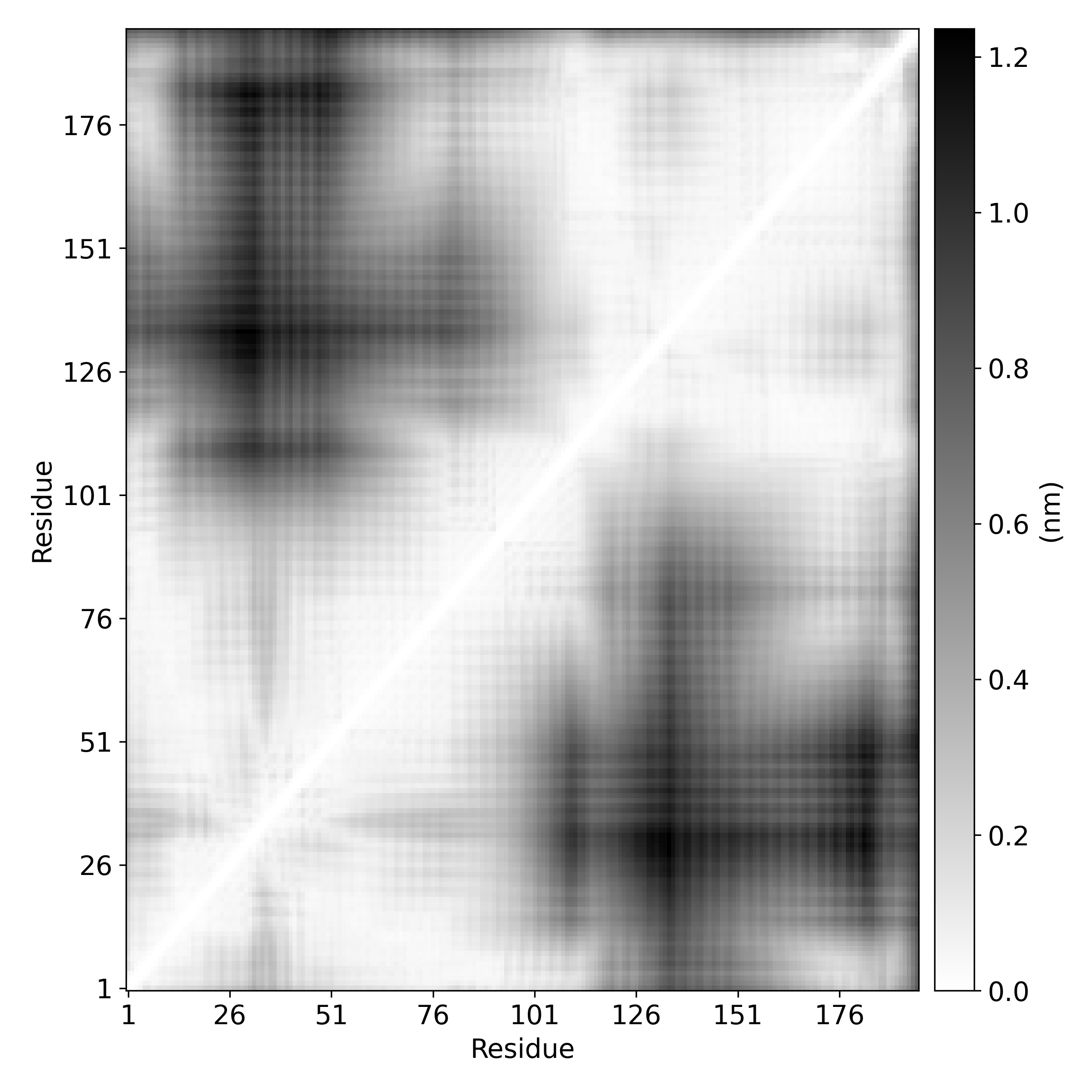
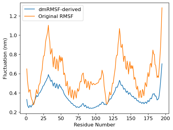
3a. Plotting distance-matrix-RMSF
Here we compare dmRMSF and conventional RMSF
We plot the standard deviation in distances in distance matrix. We use
stdev-matrix.datfile obtained fromdistmatsub-command as the input file.We calculate RMSF of the protein using
gmx rmsf
[18]:
%%bash

# Generate the dmRMSF plot
gmx_clusterByFeatures matplot -i stdev-matrix.dat -o dmRMSF-matrix.png

# Calculate the conventional RMSF
echo 3 | gmx rmsf -f inputs/woDNA.xtc -s inputs/woDNA.tpr -n inputs/index.ndx -res -o rmsf.xvg
                       :-) GROMACS - gmx rmsf, 2025.2 (-:

Executable:   /opt/gromacs-2025/bin/gmx
Data prefix:  /opt/gromacs-2025
Working dir:  /home/raj/workspace/gmx_clusterByFeatrues/tutorials/distmat-TFAM-pca
Command line:
  gmx rmsf -f inputs/woDNA.xtc -s inputs/woDNA.tpr -n inputs/index.ndx -res -o rmsf.xvg

Reading file inputs/woDNA.tpr, VERSION 4.5.5-dev-20110921-e25c350 (single precision)
Reading file inputs/woDNA.tpr, VERSION 4.5.5-dev-20110921-e25c350 (single precision)
Select group(s) for root mean square calculation
Group     0 (         System) has  3580 elements
Group     1 (        Protein) has  3580 elements
Group     2 (      Protein-H) has  1884 elements
Group     3 (        C-alpha) has   195 elements
Group     4 (       Backbone) has   585 elements
Group     5 (      MainChain) has   781 elements
Group     6 (   MainChain+Cb) has   973 elements
Group     7 (    MainChain+H) has   969 elements
Group     8 (      SideChain) has  2611 elements
Group     9 (    SideChain-H) has  1103 elements
Group    10 (    Prot-Masses) has  3338 elements
Group    11 (r_16-25_r_35-45_r_52-75_r_82-110_r_120-130_r_136-145_r_152-180) has  2331 elements
Group    12 (r_16-25_r_35-45_r_52-75_r_82-110_r_120-130_r_136-145_r_152-180_&_C-alpha) has   124 elements
Group    13 (r_1-98_&_C-alpha) has    98 elements
Group    14 (r_99-195_&_C-alpha) has    97 elements
Reading frame   32000 time 640000.000

Back Off! I just backed up rmsf.xvg to ./#rmsf.xvg.1#

GROMACS reminds you: "Being Great is Not So Good" (Red Hot Chili Peppers)
Selected 3: 'C-alpha'
3b. Deriving residue-wise fluctuation from dmRMSF
Above standard-deviation is a matrix. Therefore, to calculate fluctuations of residues, we will calculate mean of each rows. It will give the idea about fluctuations of each residue as simular to that of conventional RMSF. Subsequently, rmsf.xvg is read and plotted.
[19]:
dmRMSF = read_mat_file('stdev-matrix.dat') # read the stdev-matrix.dat file containing standard-deviation of distance matrix
derived_dmRMSF = np.mean(dmRMSF, axis=1)   # Derive the fluctuation by averaging over rows
rmsfData = read_xvg('rmsf.xvg')            # Read the conventional RMSF data

mpl.rcParams['font.size']=12
plt.plot(rmsfData[0], derived_dmRMSF, label='dmRMSF-derived')
plt.plot(rmsfData[0], rmsfData[1], label='Original RMSF')
plt.xlabel('Residue Number')
plt.ylabel('Fluctuation (nm)')
plt.legend()
plt.show()
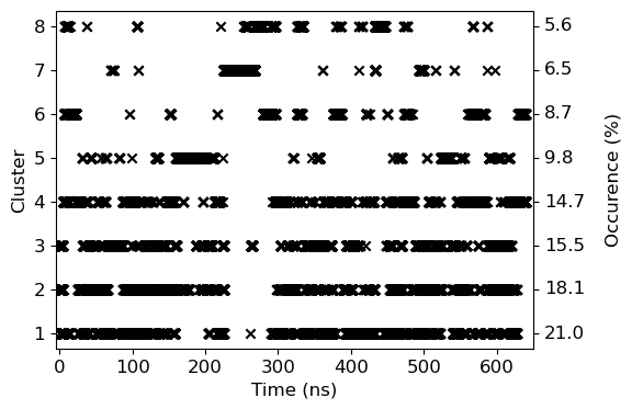
4. Cluster-ID with time
We will use clid.xvg obtained from the cluster subcommand to plot both cluster-id and also highlight the occurance of the given cluster.
[20]:
# Occurance has been calculated manually from the data obtained in cluster.log file
occur=[ 21.0, 18.1, 15.5, 14.7, 9.8, 8.7, 6.5, 5.6]

mpl.rcParams['font.size']=12

data=read_xvg('clid.xvg')
fig = plt.figure(figsize=(6,4))
fig.subplots_adjust(right=0.85)

ax = fig.add_subplot(111)
ax.scatter(data[0]/1000, data[1], marker='x', color='k')
ax.tick_params(axis='y', right=True)

ax.set_ylabel('Cluster')
ax.set_xlabel('Time (ns)')
ax.set_xlim(-5, 650)
for i in range(8):
    ax.text(665, i+1, '{0:3.1f}'.format(occur[i]), verticalalignment='center')
ax.text(760, 4.5, 'Occurence (%)', verticalalignment='center', rotation='vertical', horizontalalignment='center')

plt.savefig('clid.png', dpi=300)
plt.show()